Introduction

This work was completed by Laurent Jacques and Remi Delogne, in collaboration with Vincent Schellekens and Laurent Daudet

In the world of signal processing, we keep seeing an increase in size of signals in datasets, sometimes pushing us to resort to what we commonly refer to as sketching. The purpose of sketching is to provide a representation of a signal in a new domain, sometimes in lower dimension, while preserving essentail characteristics about it. Many applications will include sketching as a first step in data acquisition followed by a reconstruction step in order to get back the signal back in its original domain. This is similar to a wavelet transform followed by an inverse transform. However it may not always be necessary to recover the original signal, or the optimisation method hidden in the reconstruction step might prove too costly to be useful. In such cases one may wonder if acquiring information about the original signal without having explicit access to the original version is possible.

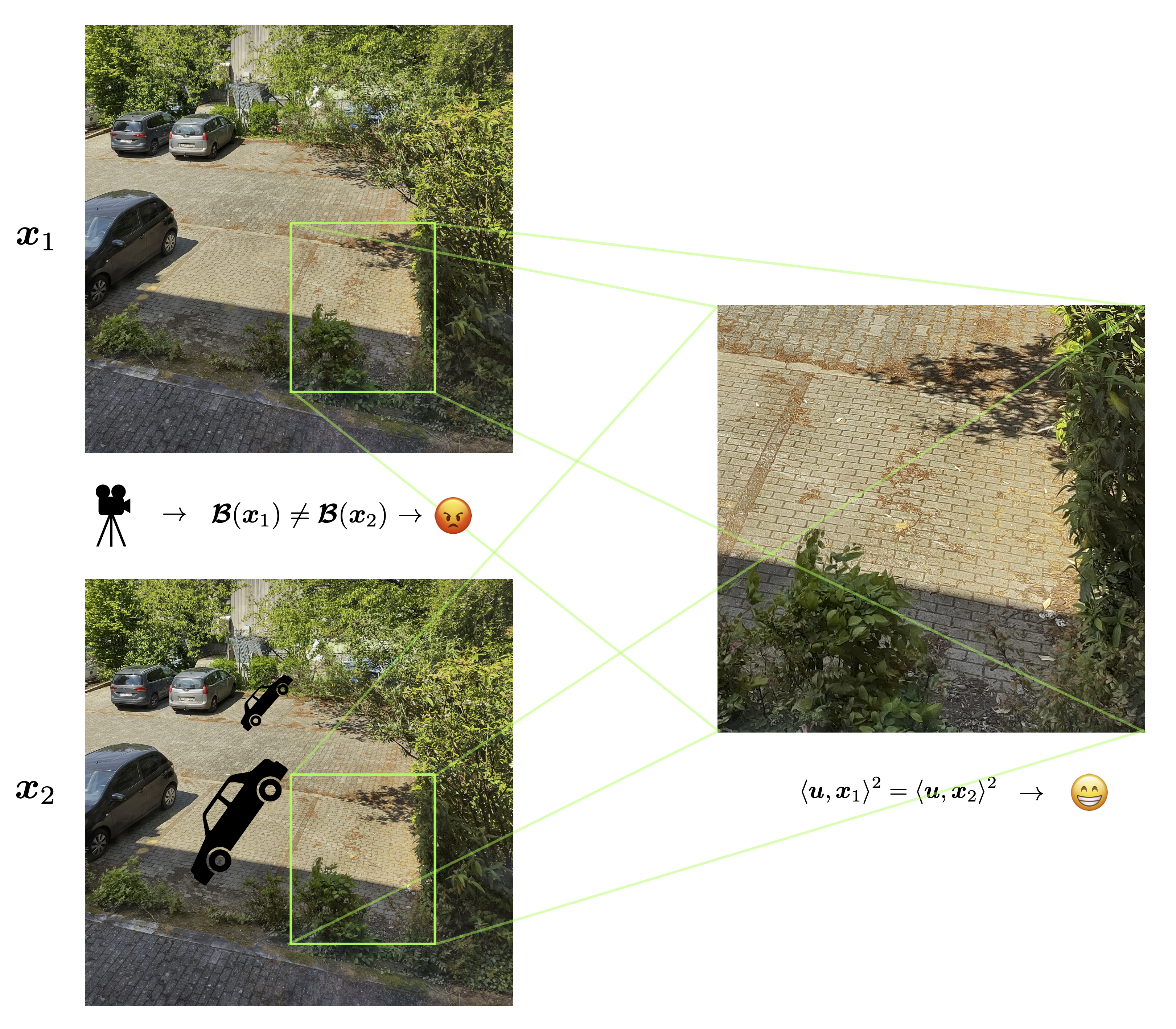
Let us think of a practical example. A surveillance camera is placed by a parking lot and records several parking spaces. For bandwidth and memory purposes the camera directly acquires images in their skethed version. I would like to know from this whether my parking space has been taken or not. This will require me to access localised information (such as the mean in a given area) about the original image only from its sketches. This is illustrated in figure 1. The image $\boldsymbol x_1$ represents the parking lot with my parking space empty, and the image $\boldsymbol x_2$ with my parking space still empty, but my neighbour’s space occupied by a new black car. Say we consider a sketching operator $\boldsymbol {\mathcal B}$. If we only look at the sketched version of both images $\boldsymbol {\mathcal B}(\boldsymbol x_1)$ and $\boldsymbol {\mathcal B}(\boldsymbol x_2)$, we will notice a difference since a new car appeared in the parking lot. However what matters to me (my parking spot) remais unchanged. If we found a way of estimating the mean value of the pixels in the area of interest, we would have an answer to our problem. This localised quantity is easy to find via a scalar product between an instance $\boldsymbol x$ and a vector $\boldsymbol u$ that contains zeros outside the area of interest and ones inside. As we will see, using the sketching described below, we will in fact be able to recover the square of the calar product between an instance and an arbitrary vector.

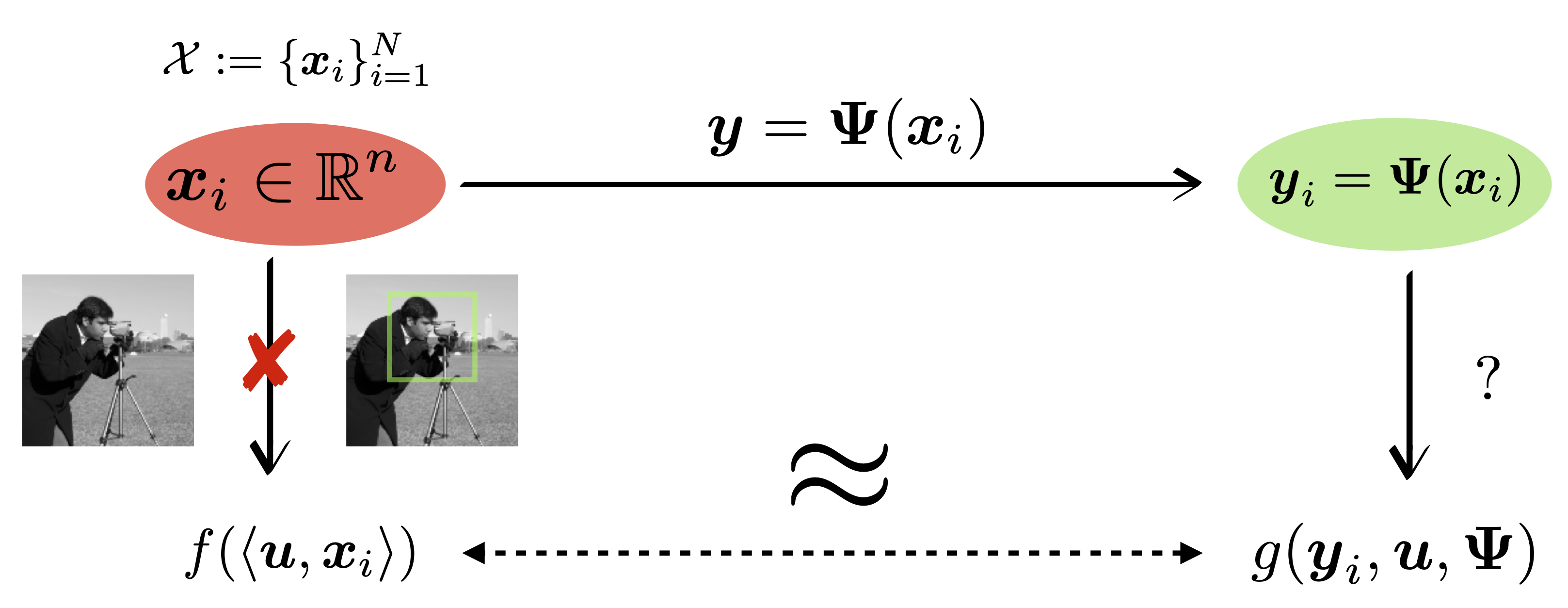
In this short piece we will show how estimating a function of this scalar product is possible, only by using the sketched version of the signals we are considering.

Sketching

Let us first briefly describe what we actually mean by sketching.

Linear sketching procedure relies on linear observations of a signal $\boldsymbol x$. Given an observation vector $\boldsymbol a_i$, a single linear observation of $\boldsymbol x$ is defined as $\boldsymbol a_i^\top\boldsymbol x$. The entire linear sketching procedure consists of a series of $m$ linear observation of $\boldsymbol x$ as illustrated in the next figure:

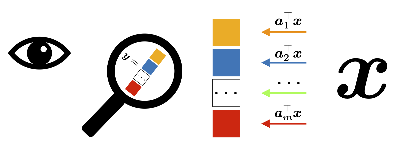
This procedure can be summarised as observing a vector via $\boldsymbol x\in\mathbb R^n$ through a matrix $\boldsymbol A\in\mathbb R^{m\times n}$ by computing $\boldsymbol y=\boldsymbol A\boldsymbol x$, the linear observations being hidden in the matrix-vector product on the right-hand-side. Notice that one can control the size of $\boldsymbol y$ by adding or removing lines to $\boldsymbol A$.

Here we focuse on a similar sketching procdure but with an added little twist. Instead of relying on linear observation of a signal of interest, we will now take the square of every linear observation. Given $\boldsymbol a_i$, one single observation is now defined as $(\boldsymbol a_i^\top\boldsymbol x)^2$ and the complete quadratic sketching procedure simply takes a series of $m$ quadratic measurements of $\boldsymbol x$:

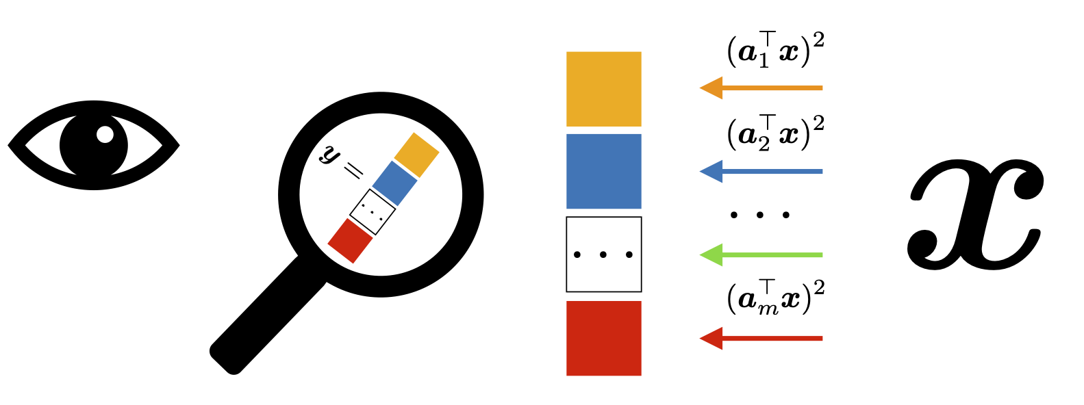
Allowing us to defie the operator $\mathcal A:\mathbb R^n\to \mathbb R^m:\boldsymbol x\mapsto \mathcal A(\boldsymbol x)=((\boldsymbol a^\top_i\boldsymbol x)^2)_{i=1}^m$. Unfortunately though, $\mathcal A$ is not isotropic meaning that the norms of its various moments is not proportional to the norms of the same moments of the original instance. But a simple solution exists: $\mathcal B:\mathbb R^n\to\mathbb R^m:\boldsymbol x\mapsto\mathcal B(\boldsymbol x)=((\boldsymbol a^\top_{2i+1} \boldsymbol x)^2-(\boldsymbol a_{2i}^\top\boldsymbol x)^2)_i^m$ which is isotropic and as is required to prove the next result.

Signal Processing

Remember that in the introduction we described how we wanted to evaluate a scalar product between the instance and another vector. Well it turns out that if we define a vector $\boldsymbol u$ fit for our purposes, we can estimate $\langle \bolsymbol u,\boldsymbol x\rangle$ arbitrarily well provided that $m$ is large enough.

More precisely, given a unit vector $\boldsymbol y \in \mathbb R^n$, $\kappa = \pi/4$, and a distortion $0<\delta <1$, provided that $m \geq C \delta^{-2} k \log(\frac{n}{k\delta})$, then, with probability exceeding $1 - C \exp(-c \delta ^2 m)$, we have for all $k$-sparse signals $\boldsymbol x$,

$$\textstyle \Big|\frac{\kappa}{m} \langle \mathcal B(\boldsymbol x),\text{sign}(\mathcal B(\boldsymbol y))\rangle - {\langle\boldsymbol x,\boldsymbol y\rangle^2} \Big| \leq \delta |\boldsymbol x|^2.$$

In words this states that we can approximate the squared dot product between an instance $\boldsymbol x$ and a unit vector $\boldsymbol u$ by taking the sign of the sketch of $\boldsymbol u$ and projecting the sketch of $\boldsymbol x$ on it.

We refer to this result as the sign product embedding or SPE.

Experiments

Interstingly, a special optical computer (Optical Processing Unit, or OPU) developped by the startup LightOn is capable of approximating $\mathcal A(\boldsymbol x)$ with $m$ up to 1.000.000 provided that $\boldsymbol x$ is binary. Without going into details, a few tweaks allow us to replicate the operator $\mathcal B$ “At the speed of light” (a telling metaphor since the OPU literally transforms instances into a light beam to replicate the numerical operation that would otherwise be performed on a computer).

To demonstrate the quality of our approach and the potential practical uses of the OPU, we designed a few toy experiments described here:

Event detection

Consider the situation of a video stream feeding one image of a white rotating disk per time step. Echoing the practical situation with the parking lot in the introduction, we would like to design a event detection algorithm that is capable of telling when the disk is going through one particular quadrant of the image (see figure 4), assuming we only have access to the sketches of the images.

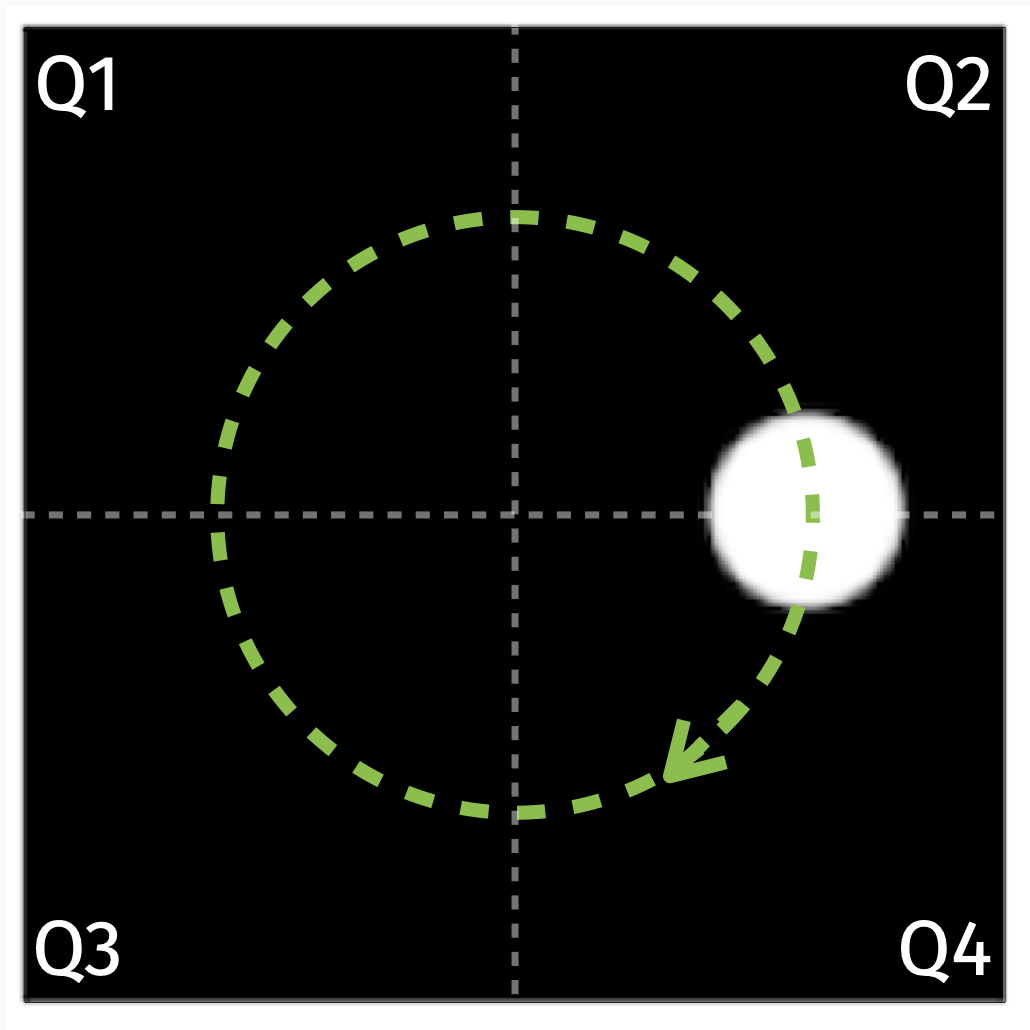
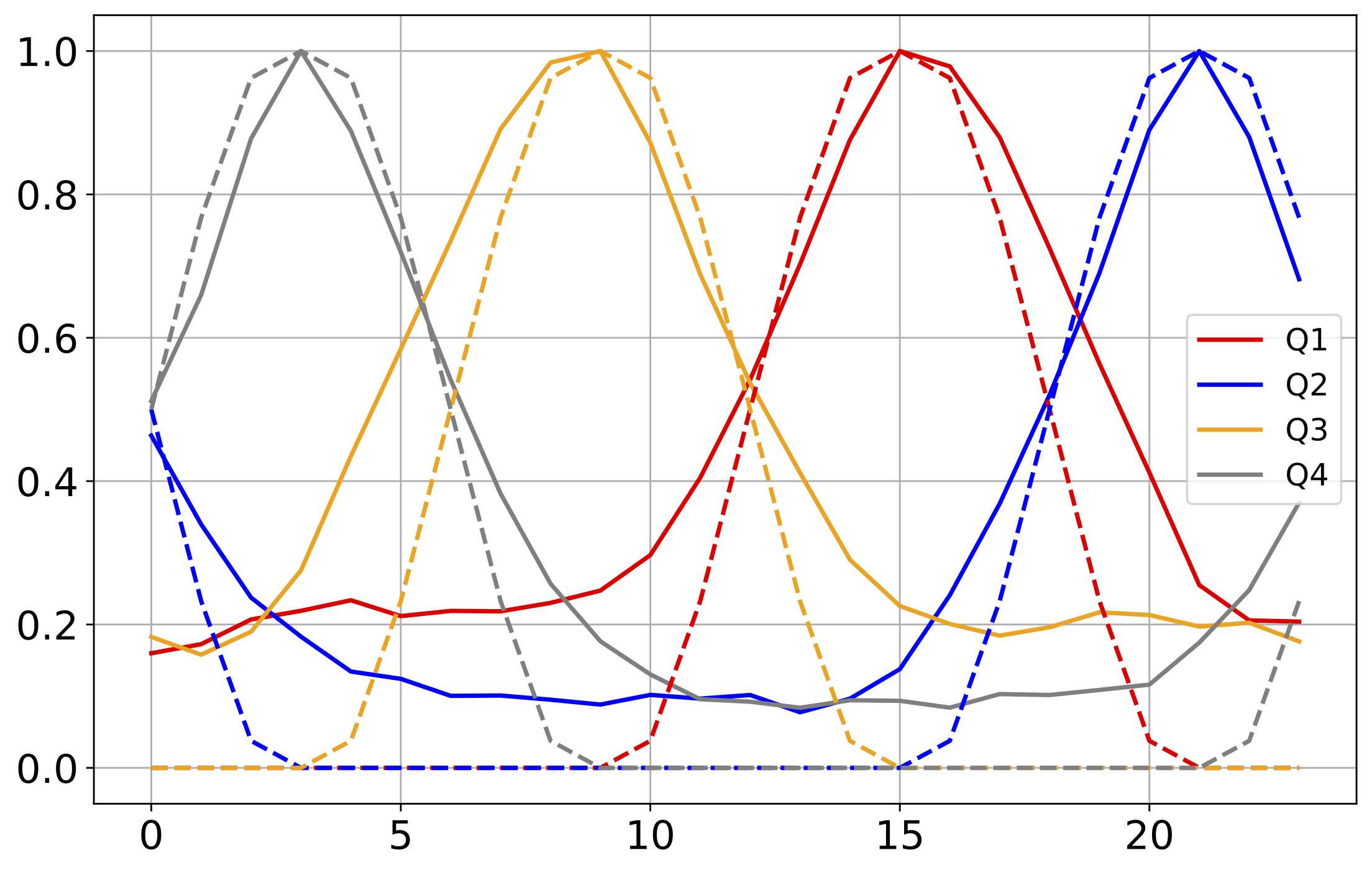
We used our SPE approximation with vectors $\boldsymbol u_1,\boldsymbol u_2,\boldsymbol u_3,\boldsymbol u_4$ (for every quadrant) designed with zeros outside their assigned quadrants in order to give us an approximation of the square of the averge pixel value in every quadrant for every time step. The normalised results are displayed in figure 5, where we can clearly see the patterns of the circle moving through the image. There were 24 images of size 950$\times$950, sketched using the OPU to simulate $\cl B$ with $m=10.000$.

MNIST Naive classification of sketched test instances

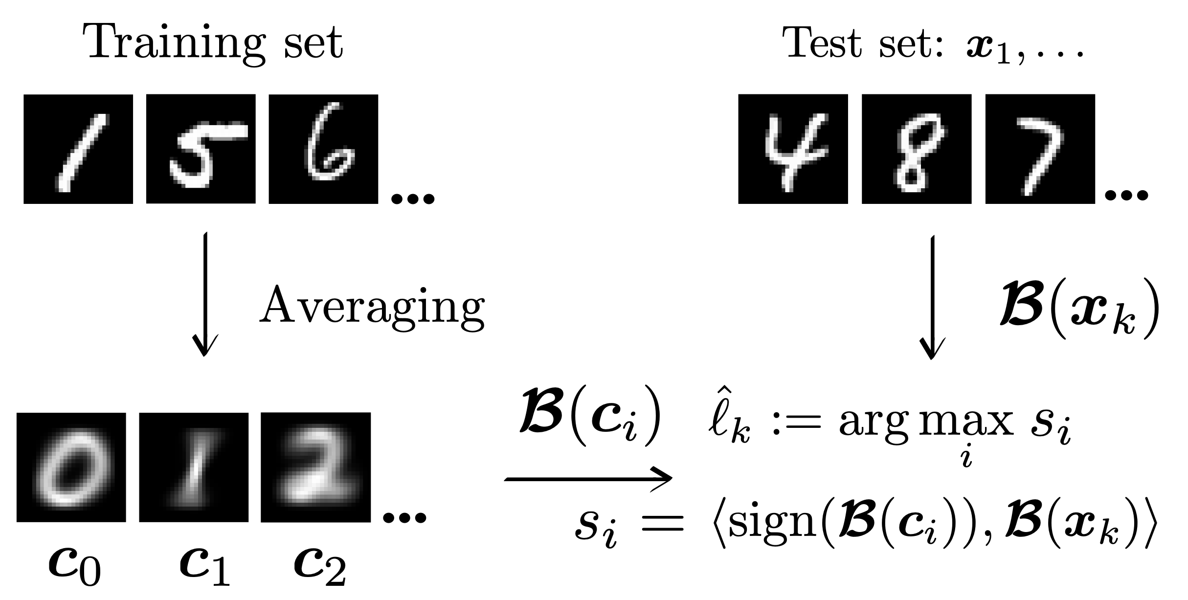
In this experiment we developped a very naive classification algorithm for MNIST. We first take every class of instance in the training set and create an average image $\boldsymbol c_i$ for every class $j$ (also known as a centroid). We then classified the test data by evaluating the scalar product between a new instance $\boldsymbol x_k$ and every centroid $\boldsymbol c_j$ and assigning the estimated class $\hat l_k$ of the new instance to the same as that of the centroid yielding the highest scalar product. In order to test the SPE and the OPU, we the repeated the experiment by first creating the centroids, then sketching those centroids and comparing them to the sketches of the instances of the test set. The whole procedure is summariseed in figure 5:

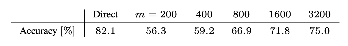
We obtained the following results for various values of $m$ (and with the result in the direct domain for reference):

MNIST classification in the sketched domain

In this experiment we repeated the same setup as the previous experiment but this time starting with a sketched dataset from which we created the centroids $\boldsymbol c_j^{\mathcal B}$ to then compare them to sketched test instances $\mathcal B(\boldsymbol x_k)$ to get an estimated class $\hat l_k$ for $\boldsymbol x_k$. This procedure is summarised in figure 6:

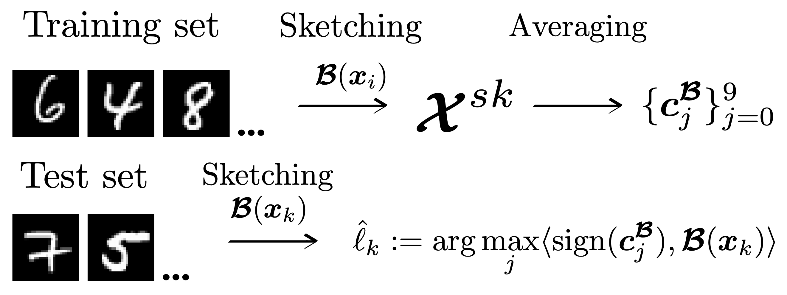
Interestingly, using $m=10.000$ we got a classification accuracy of $82.7$% which slightly outperforms the accuracy of the direct domain of $82.1$%.

Conclusion

We have shown that in the context of quadratic sketching, it is possible to estimate functions of sketched signals without reconstructing them with boring and costly optimisation methods up to a controlled distortion. More detilas about these results can be found here¹ and here².