Bilinear and Biconvex Inverse Problems for Computational Sensing Systems
Recent years have been characterised by a surge of efforts into new computational sensing modalities, i.e., signal, image and tensor sampling strategies in which signal processing plays a central role in forming an estimate of the signal being measured, $\boldsymbol x$. While computational sensing is, by itself, largely used in practice (in fact, most medical imaging strategies are based on such principles), its resurgence in other computational imaging modalities is mainly due to theoretical advances in the solution of inverse problems, as well as computational advances in large-scale data processing.
In particular, for many inverse problems arising in the acquisition of natural and man-made signals, the principle of sparsity has changed the way we approach them; in addition, the theory of compressed sensing – in which sparsity is related to the intrinsic properties of the sampling operator and the signal itself – has provided a very general framework for the design of new sensing modalities.
However, the physical implementation of computational sensing strategies is far from being simple or stable, and is a subject of ongoing research. Since the inverse problem that maps the measurements collected by the sensing device to an estimate of the original signal typically requires a very accurate numerical model of the physical sensing system, it is often the case that non-trivial calibration procedures are required to complete or refine the available information describing the sensing system.
In general terms, if the sensing system is represented by a linear operator $\mathcal A$ that produces some measurements $\boldsymbol y = \mathcal A(\boldsymbol x)$, it is often the case that there is a mismatch between the model $\mathcal A$ and its implementation $\mathcal A_{\boldsymbol t}$, that is $\boldsymbol y = \mathcal A_{\boldsymbol t}(\boldsymbol x) \neq \mathcal A (\boldsymbol x)$ where the missing parameters $\boldsymbol t$ are part of the unknowns and are actually mixed with the signal. Rather than using known training signals $\boldsymbol x$ to fix part of the unknowns in $\boldsymbol y = \mathcal A_{\boldsymbol t}(\boldsymbol x)$ and be able to retrieve $\boldsymbol t$, we focus on what are commonly referred to as a blind approaches, i.e., when both $\boldsymbol t$ and $\boldsymbol x$ are missing and should be estimated jointly.
Even more generally, the sensing operator $\mathcal A$ could be quadratic with respect to the signal it is applied to, as is the case in phase retrieval (Candes, Li, Soltanolkotabi 2015).
The common aspect of such a broad class of sensing models is in that, when we attempt to solve the inverse problem
$$(\hat{\boldsymbol x}, \hat{\boldsymbol t}) := {\rm argmin}_{(\boldsymbol \xi, \boldsymbol \theta) \in \mathbb D_{\boldsymbol \xi} \times \mathbb D_{\boldsymbol \theta}} f(\boldsymbol \xi, \boldsymbol \theta)$$
that minimises the discrepancy $$f(\boldsymbol \xi, \boldsymbol \theta) := |\boldsymbol y - \mathcal A_{\boldsymbol \theta}(\boldsymbol \xi)|^2_2$$ between the observations and the solution
on some domain $\mathbb D_{\boldsymbol \xi} \times \mathbb D_{\boldsymbol \theta}$ we are faced with a non-convex objective function and optimisation problem, which is well-known to lack the beneficial properties and broadly applicable solution frameworks available for smooth as well as non-smooth convex problems.
In this branch of our research on sensing and imaging we aim at addressing such non-convex objectives $f(\boldsymbol \xi, \boldsymbol \theta)$ under a randomisation, i.e., when the sensing operator features a fully random part that allows to produce, from one (or more) unknown input $\boldsymbol x$ and set of parameters $\boldsymbol t$, several realisations of $\boldsymbol y$. In particular, we aim at analysing problems for which, when taken in expectation with respect to some random vector (or matrix elements) $\boldsymbol a$, our objective function is so that
$$ f(\boldsymbol \xi, \boldsymbol \theta) \simeq \mathbb E_{\boldsymbol a} f(\boldsymbol \xi, \boldsymbol \theta)$$
is actually convex, but only under an asymptotic regime with respect to $\boldsymbol a$, that is if we had potentially infinite observations as an input to our inverse problem/estimator.
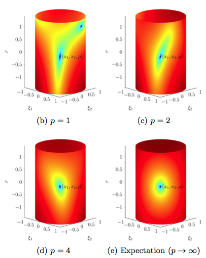
Intuitively and roughly speaking, if even in such an infinite-sample regime the problem is non-convex, there is no hope of solving it with simple methods; conversely, if there exists a non-asymptotic regime for which which we can bound
$$\vert f(\boldsymbol \xi, \boldsymbol \theta) - \mathbb E_{\boldsymbol a} f(\boldsymbol \xi, \boldsymbol \theta) \vert \leq \delta$$
for some arbitrarily small $\delta$, it is sensible that the optimisation problem will be (at least locally) convex, and enjoy for finite-sample regimes of the properties of the problem in expectation.
With this rationale in mind we mention, among others, many recent breakthroughs in the context of phase retrieval (Candès, Strohmer, Voroninski 2014; Candès, Li, Soltanolkotabi, 2015; White, Sanghavi, Ward, 2015; Sun, Qu, Wright, 2016), covariance estimation and sketching (Chen, Chi, Goldsmith 2015), blind deconvolution and demixing (Ahmed, Recht, Romberg, 2014; Ahmed, Cosse, Demanet, 2015; Bahmani and Romberg, 2015; Ling and Strohmer 2016; Li, Ling, Strohmer, Wei 2016) as well as blind calibration (Friedlander and Strohmer 2014; Ling and Strohmer 2015; Cambareri and Jacques 2016). The most important aspect of such approaches with respect to the previous literature (e.g., Balzano and Nowak 2008; Bilen, Puy, Gribonval, Daudet, 2014) is in that they are endowed with recovery guarantees, rigorous requirements which grant that the above optimisation problem actually yields the exact solution.
Note that some of these works adopt a convexification of the corresponding inverse problem, and in doing so often resort to lifting it to a higher-dimensional, large-scale version that can be computationally challenging. In our research, we focused on blind calibration for imaging systems based on compressed sensing, and have advocated the use of non-convex algorithms for the solution of such non-convex problems without convexification. As is typically the case, the solution passes through a two-step procedure involving the choice of an initialisation point and a descent algorithm from such an initialiser; as for the theory, the general outline involves ensuring the initialisation point falls in a small neighbourhood of the exact solution, and that the gradients of our objective $f(\boldsymbol \xi, \boldsymbol \theta)$ are well-behaved thanks to their (non-asymptotic) behaviour, that is as close as required to the asymptotic case in the number of samples.
In addition, when sparsity or low-dimensional models (e.g., subspace models) hold on either or both $\boldsymbol x$, $\boldsymbol t)$, it is possible to simplify the estimation according to such priors. These different scenarios have been tackled in our contributions.
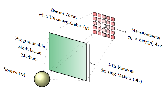
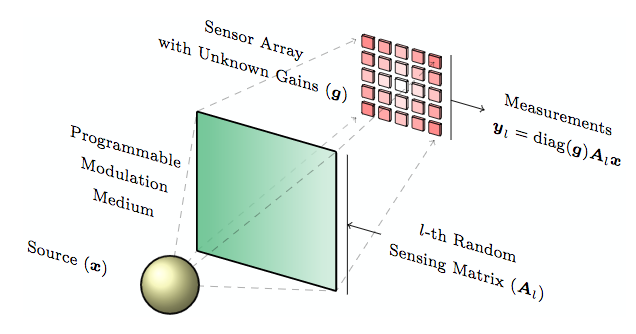
In particular, we have focused on a special instance of blind calibration, that is solving the bilinear system
$$\boldsymbol y_l = {\rm diag}({\boldsymbol g}) {\boldsymbol A}_l {\boldsymbol x}, \ l = 1, \ldots, p$$
in $(\boldsymbol x, \boldsymbol g)$ where ${\boldsymbol A}_l \in \mathbb R^{m \times n}$ are independent and identically distributed (i.i.d.) random matrices with i.i.d. sub-Gaussian entries. In this case, we have solved
$$ \mathop{{\rm argmin}}_{({\boldsymbol \xi},{\boldsymbol \gamma}) \in \Sigma \times {\mathcal B}} \textstyle\frac{1}{2mp} {\sum_{l=1}^{p} \left\Vert {\rm diag}({\boldsymbol \gamma}) {\boldsymbol A}_l {\boldsymbol \xi} - \boldsymbol y_l\right\Vert^2_2} $$
where $\Sigma \subseteq \mathbb R^n$ is a subspace of a signal domain and $\mathcal B \subset \mathbb R^m$ is a closed convex set of gains (assumed positive).
When $\boldsymbol g$ is not too far from unity (i.e., it is in a sense not too peaky) but still significantly different from it as to require calibration, we have found a setup and simple framework for gradient descent-based algorithms – as described in our contributions – that are actually capable of converging under a requirement in the number of samples that scales (up to some simplifications) as
$$m p = {\mathcal O}((\dim \Sigma + \dim \mathcal B) \log^2 m(p+n)).$$
Moreover, when $\Sigma$ is a union of canonical subspaces (i.e., for sparse signals $\boldsymbol x$) we have found reassuring numerical evidence that the insertion of a hard thresholding step in our former algorithm still provides convergence provided that we operate in the proper region of the empirical phase transition (with respect to the observations $mp$) of this algorithm, whose theoretical guarantees are being explored.
In conclusion, we believe that this research, and its potential extension to blind deconvolution is critical for compressive imaging strategies, which are essentially hindered by the realisation of the sensing operator in the physical domain, and whose mismatch with the mathematical model often takes the form of a convolution kernel (i.e., blind deconvolution) or of some unknown gains per collected measurement (i.e., blind calibration); the algorithms and methods we propose then aim at avoiding all calibration phases (which are typically “non-compressive” and carried out off-line) to attain more robust and agile compressive imagers.
References:
a) Own Contributions:
-
2016. “Through the Haze: A Non-Convex Approach to Blind Calibration for Linear Random Sensing Models”, V. Cambareri and L. Jacques, Submitted to Information and Inference: A Journal of the IMA, arXiv:1610.09028
-
2016. “A Greedy Blind Calibration Method for Compressed Sensing with Unknown Sensor Gains”, V. Cambareri and L. Jacques, Submitted to ICASSP'17, arXiv:1610.02851
-
2016. “Non-Convex Blind Calibration for Compressed Sensing via Iterative Hard Thresholding”, V. Cambareri, L. Jacques, Accepted in the 11th IMA International Conference on Mathematics in Signal Processing, Birmingham, UK (12-14/12/2016), dial:2078.1/178320
-
2016. “A Non-Convex Blind Calibration Method for Randomised Sensing Strategies”, V. Cambareri, L. Jacques, 2016 4th International Workshop on Compressed Sensing Theory and its Applications to Radar, Sonar and Remote Sensing (CoSeRa) (invited), arXiv:1605.02615, doi:10.1109/CoSeRa.2016.7745690, dial:2078.1/178303
-
2016. “A Non-Convex Approach to Blind Calibration for Linear Random Sensing Models”, V. Cambareri, L. Jacques, Proceedings of the “international Traveling Workshop on Interactions between Sparse models and Technology (iTWIST'16)”, Aalborg, Denmark, 2016, arXiv:1609.04167, dial:2078.1/178307
-
2016. “A Non-Convex Approach to Blind Calibration from Linear Sub-Gaussian Random Measurements”, V. Cambareri and L. Jacques , 37th WIC Symposium on Information Theory in the Benelux, 6th joint WIC/IEEE SP Symposium on Information Theory and Signal Processing in the Benelux, dial:2078.1/178326
b) Related Work:
-
Ahmed, Ali, Augustin Cosse, and Laurent Demanet. “A convex approach to blind deconvolution with diverse inputs.” Computational Advances in Multi-Sensor Adaptive Processing (CAMSAP), 2015 IEEE 6th International Workshop on. IEEE, 2015.
-
Ahmed, Ali, Benjamin Recht, and Justin Romberg. “Blind deconvolution using convex programming.” IEEE Transactions on Information Theory 60.3 (2014): 1711-1732.
-
Ahmed, Ali, Felix Krahmer, and Justin Romberg. “Empirical Chaos Processes and Blind Deconvolution.” arXiv preprint (2016).
-
Bahmani, Sohail, and Justin Romberg. “Lifting for blind deconvolution in random mask imaging: Identifiability and convex relaxation.” SIAM Journal on Imaging Sciences 8.4 (2015): 2203-2238.
-
Balzano, Laura, and Robert Nowak. “Blind calibration of sensor networks.” Proceedings of the 6th international conference on Information processing in sensor networks. ACM, 2007.
-
Bilen, Çağdaş, et al. “Convex optimization approaches for blind sensor calibration using sparsity.” IEEE Transactions on Signal Processing 62.18 (2014): 4847-4856.
-
Candes, Emmanuel J., Thomas Strohmer, and Vladislav Voroninski. “Phaselift: Exact and stable signal recovery from magnitude measurements via convex programming.” Communications on Pure and Applied Mathematics 66.8 (2013): 1241-1274.
-
Candes, Emmanuel J., Xiaodong Li, and Mahdi Soltanolkotabi. “Phase retrieval via Wirtinger flow: Theory and algorithms.” IEEE Transactions on Information Theory 61.4 (2015): 1985-2007.
-
Chen, Yuxin, Yuejie Chi, and Andrea J. Goldsmith. “Exact and stable covariance estimation from quadratic sampling via convex programming.” IEEE Transactions on Information Theory 61.7 (2015): 4034-4059.
-
Friedlander, Benjamin, and Thomas Strohmer. “Bilinear compressed sensing for array self-calibration.” 2014 48th Asilomar Conference on Signals, Systems and Computers. IEEE, 2014.
-
Li, Xiaodong, et al. “Rapid, robust, and reliable blind deconvolution via nonconvex optimization.” arXiv preprint arXiv:1606.04933 (2016).
-
Ling, Shuyang, and Thomas Strohmer. “Blind deconvolution meets blind demixing: Algorithms and performance bounds.” arXiv preprint arXiv:1512.07730 (2015).
-
Ling, Shuyang, and Thomas Strohmer. “Self-calibration and biconvex compressive sensing.” Inverse Problems 31.11 (2015): 115002.
-
Ling, Shuyang, and Thomas Strohmer. “Self-Calibration via Linear Least Squares.” arXiv preprint arXiv:1611.04196 (2016).
-
Sanghavi, Sujay, Rachel Ward, and Chris D. White. “The local convexity of solving systems of quadratic equations.” Results in Mathematics (2016): 1-40.
-
Sun, Ju, Qing Qu, and John Wright. “A geometric analysis of phase retrieval.” arXiv preprint arXiv:1602.06664 (2016).
c) Available Presentations (pdf slides):
- 2016 “Towards Non-Convex Blind Calibration for Compressed Sensing”, FNRS Wavelet Contact Group, 16 November 2016